
2022 Workshop on Molecular Evolution at the MBL
Follow this link to go to back to workshop schedule page.
Follow this link to go to back to the Bielawski faculty page.
The objective of this activity is to help you understand how to use different codon models, and how to test for selection using PAML (and specifically the CODEML program). The activities are designed to build general analytical skills, and are just as relevant to analyses carried out using other software packages, such as HyPhy.
The tutorial is divided into 4 exercises.
NOTE: Beginning in 2023, in The Workshop on Molecular Evolution we will ONLY do excercises 1, 3 & 4. This includes the optional step (No. 8) of excercise 4.
The next section (Accessing the files) describes how to access and work with the files required for each of the exercises. You will access the files differently depending on whether you are doing the labs at the workshop or at home independently of the workshop.
Note that running the program involves modifying input files and creating output files. It is best practice to (i) create a separate directory for each exercise or real-data analysis that you want to do and (ii) record and save simple-text notes about the motivation and details of each real-data analysis and store them within the directory that created for each analysis. The latter is a kind of “read me” file that you will be glad to have after you have done many analyses on your real data and have begun to forget, or mix up, the details.
Here are the slides for the PAML learning activity: slides
Here is a copy of the book chapter that accompanies these exercises: Book_Chapter.pdf
This page has links to useful documents and many additional resources.
1. If you are doing the lab AT THE WORKSHOP: On the virtual machines we will be using in the 2022 workshop, there will be a symlink in your home directory named "moledata" that takes you to the course data files. There you will find directories for the various labs (e.g., MSAlab, revbayes, PamlLab, etc.).
To view the list of labs type:
ls ~/moledata
To view the contents of the Paml Lab type:
ls -1 ~/moledata/PamlLab
This will reveal the directories for each excercise:
ex1
ex2
ex3
ex4
The files are already on the virtual machine you are using. However, you will want to run each exercise in a separate directory that you will create. So, create a new directory. The name of the new directory is up to you, but pick something informative (e.g., ~/PAML_ex1).
To copy the files required for exercise 1 just type:
cp ~/moledata/PamlLab/ex1/* ~/PAML_ex1
Now you are ready to do exercise 1 within ~/PAML_ex1
2. Renaming files: For all exercises you will need to rename the control file by removing the exercise (exN) prefix. You can do this by using the cp command.
Here is an example for exercise 1:
cp ex1_codeml.ctl codeml.ctl
WARNING: Re-running PAML within a directory will overwrite all files within that directory! Make sure you rename all files you want to keep!
3. If you are doing the lab INDEPNDENTLY of the workshop: You can do this lab by downloading all the necessary files from an archive here, or you can download the files individually for each exercise as you need them here.
Either way, it is still "best practice" to run each exercise in a separate working directory that you will create (e.g., PAML_ex1), and work with copies of the required files within that directory.
The objective of this activity is to use CODEML to evaluate the likelihood of the GstD1 sequences for a variety of ω values. Plot log-likelihood scores against the values of ω and determine the maximum likelihood estimate of ω. Check your finding by running CODEML’s hill-climbing algorithm.
Find the input files for Exercise 1 (ex1_codeml.ctl, seqfile.txt) and familiarize yourself with them. Pay close attention to the contents of the modified control file called ex1_codeml.ctl.
Remember to create a directory where you want your results to go, and place all your files within it. Now open a terminal, move to the directory that contains your files. When you are ready to run CODEML, delete the ex1_ prefix (the control file must be called codeml.ctl). Now you can run CODEML.
Familiarize yourself with the results (see annotations in ex1_HelpFile.pdf). If you have not edited the control file the results will be written to a file called results.txt. Identify the line within the results file that gives the likelihood score for the example dataset.
Now change and save the control file and re-run CODEML for a different fixed value of ω. The control file "quick guide" might be helpful here (quick guide). The objective is to compute the likelihood of the example dataset given a fixed value of ω. Change the control file as follows:
Change the name of your result file (via outfile= in the control file) or you will overwrite your previous results!
Change the fixed value for omega by changing the value for omega= in the control file. The values for this exercise are provided as comments at the bottom of the example control file that has been provided to you.
Repeat Step 4 for each value of ω according to the comments of the example control file (e.g., ω = 0.005, 0.01, 0.05, 0.1, 0.2, 0.4, 0.8, 1.6, 2.0).
Use your favorite spread sheet or statistical package to plot the likelihood score (y-axis) against the fixed value for omega (x-axis). Use a logarithmic scale for the x-axis (do not transform ω). Your figure should look something like this: ex1 plot template.pdf (note: the data points have been intentionally omitted from this version of the plot; you need to generate the data for yourself).
From your plot, try to answer this question:
Now change the control file so that CODEML will use its hill-climbing algorithm to find the MLE; set fix_omega=0 in the control file. Compare the result to your guess from Step 7.
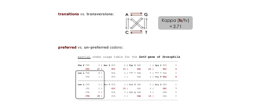
in this exercise you will investigate the sensitivity of ω to the transition/transversion ratio (kappa), and to the assumed codon frequencies (π's). After you collect the required data you will determine which assumptions yield the largest and smallest values of S, and what effect it has on the value of ω.
Find the files for Exercise 2 (ex2_codeml.ctl, seqfile.txt) and familiarize yourself with them. It would be best to create a new directory for Exercise 2. When you are ready to run CODEML, delete the ex2_ prefix (the control file must be called codeml.ctl).
Run CODEML using the settings in the control file for Exercise 2. Familiarize yourself with the results (ex2 HelpFile.pdf). In addition to the likelihood score you must be able to identify the part of the result file that provides estimates of the following:
Number of synonymous or nonsynonymous sites (S and N))
Synonymous and nonsynonymous rates (dS and dN)
As in Exercise 1, you will need to change and save the control files and re-run CODEML. The control file "quick guide" might be helpful here (quick guide).The objective is to compute the likelihood of the example dataset under different model assumptions. To do this you must:
Change the name of the main result file (via outfile= in the control file) or you will overwrite your previous results
Change the model assumptions about codon frequencies (via CodonFreq=) and kappa (via kappa= and fix_kappa=).
Repeat step 3 for each set of assumptions about codon frequencies and kappa given as comments at the bottom of the example control file, and shown in the figure below.

In your favorite spreadsheet program create a table like Table E2 in the slides (see ex2 table template.pdf) and fill it in with your results.
Use your table to determine:
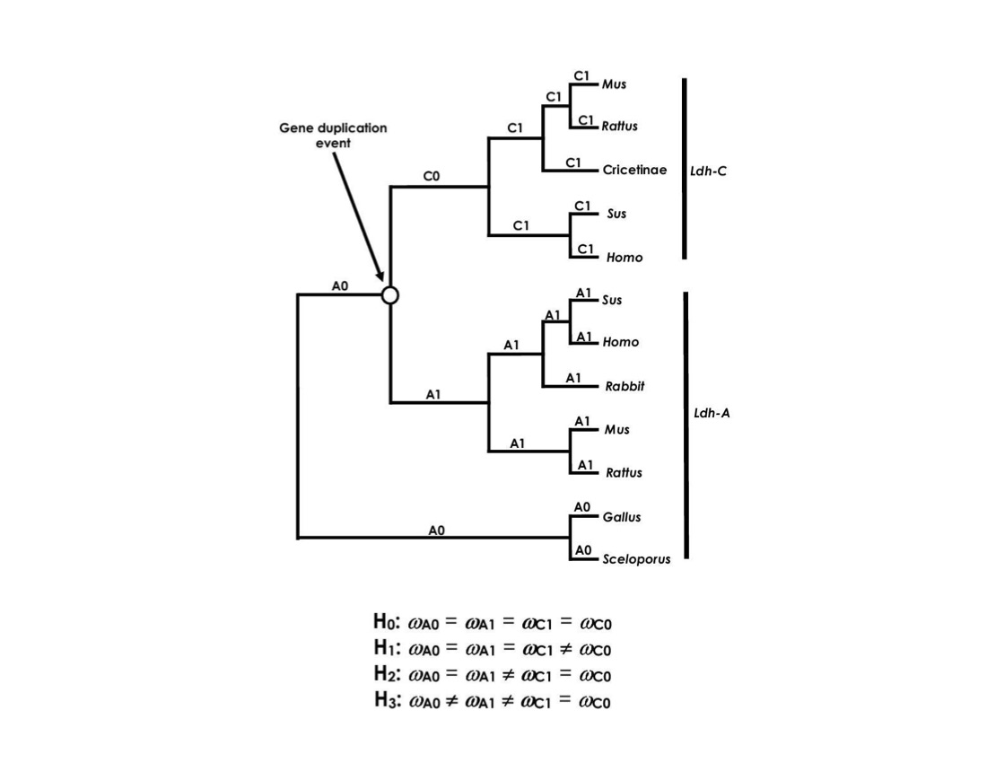
The objective of this exercise is to use three LRTs to evaluate the following possibilities: (1) the mutation rate of Ldh-C has increased relative to Ldh-A, (2) a burst of positive selection for functional divergence occurred following the duplication event that gave rise to Ldh-C, and (3) there was a long term shift in selective constraints following the duplication event that gave rise to Ldh-C.
Obtain the files for Exercise 3 from the course web-site (ex3_codeml.ctl, seqfile.txt, treeH0.txt, treeH1.txt, treeH2.txt, treeH3.txt). The tree files represent different hypotheses denoted H0, H1, H2 & H3 (see diagram below, or download this file genetree). These evolutionary concepts described above are covered by these four precise hypotheses:
H0: Homogeneous selection pressure over the tree (concept = any rate differences are due to changes in mutation rate).
H1: Episodic change in selection pressure in Ldh-C (concept = only in the branch that immediately follows the gene duplication event).
H2: A long term shift in selection pressure in Ldh-C only (concept = Ldh-C has a novel selection pressure, as compared to its ancestors, whereas Ldh-A remains subject to the ancestral level of selection pressure).
H3: A long term shift in selection on both Ldh-C and Ldh-A (concept = both paralogous lineages experience novel selection pressures; i.e., different from each other, and from the ancestor).
Run CODEML using the settings in the control file for Exercise 3. Familiarize yourself with the results (ex3_HelpFile.pdf). In addition to the likelihood score you must be able to identify the branch-specific estimates of the ω parameter. (In the first run, the branch specific values for ω will all be the same. In later runs there will be differences among some branches).
As in the previous exercises, you will need to change the control file and re-run CODEML. The control file "quick guide" might be helpful here (quick guide).The objective is to compute the likelihood, and estimate ω parameters, under different models of how selection pressure changes in different parts of the tree. Because the relevant model information is contained in the tree file, you will need specify one of several tree files in each analysis, and change the control file so that it reads the required tree file.
As always, you should change the name of the main result file (via outfile= in the control file) or you will overwrite your previous results.
Change the model assumptions about branch specific ω values by changing the tree files (via treefile= and model=) set within the control file.
Repeat step 3 for each of the four tree files that have been provided to you. Again, keep track of your results by using a table like Table E3 shown in the slides (see ex3 table template.pdf). In addition, carry out likelihood ratio tests (LRT) of the hypotheses below. See the lecture notes for additional details about LRTs. Use 1 degree of freedom to obtain the P-value for each LRT. (Helpful for computing the P-value: Chi-Square calculator
LRT statistic = 2(lnLHA - lnLH0)
Do the following LRTs, each with df=1.
Use your table of results to determine:
Which model(s) are supported by the data?
What biologcial scenario is the best explanation of Ldh gene-family evolution?
Is there evidence of positive selection during the history of Ldh evolution?
Are there any scenarios in which Ldh could have evolved by positive selection that would be undetectable by these LRTs?
The objective of this exercise is to use a series of LRTs to test for sites evolving under positive selection in the nef gene. If you find significant evidence for positive selection, then identify the involved sites by using empirical Bayes methods.
Obtain all the files for Exercise 4 (ex4_codeml.ctl.txt, ex4_seqfile.txt, treeM0.txt, treeM1.txt, treeM2.txt, treeM3.txt, treeM7.txt, treeM8.txt). When you are ready to run CODEML, remember to delete the ex4_ prefix (the control file must be called codeml.ctl).
If you plan to run two or more models at the same time, then create a separate directory for each run and place a copy of the sequence file, and the required control file and tree file in each directory.
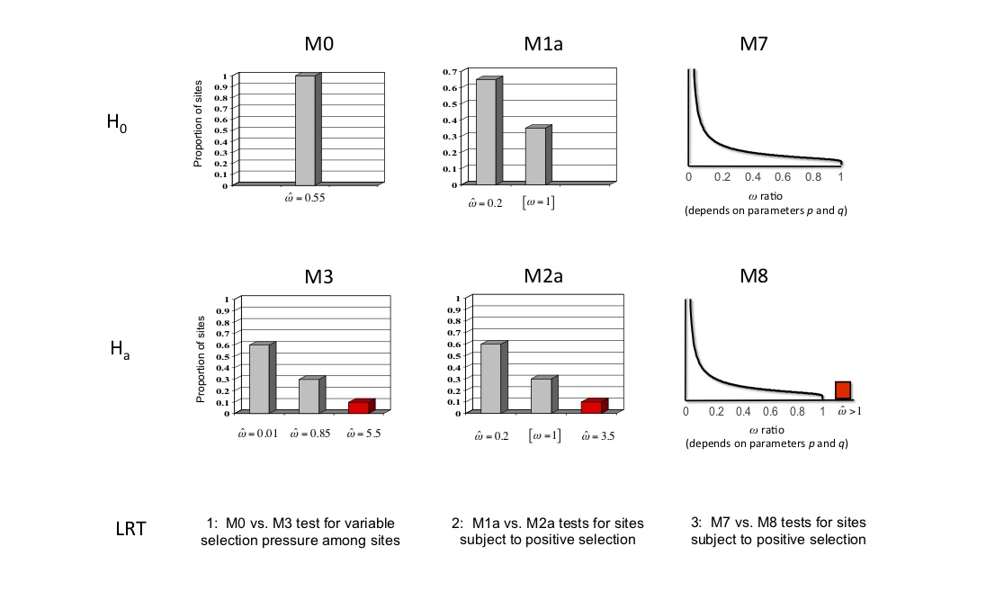
As in all the previous exercises, you will need to change the control file and re-run CODEML several times. In this case you will be fitting six different codon models (M0, M1a, M2a, M3, M7 & M8) to the example dataset. The control file "quick guide" might be helpful here (quick guide).
If you are running your analyses sequentially in the same directory, then you should change the name of the main result file (via outfile= in the control file) or you will overwrite your previous results.
Set the tree file with treefile=. I have supplied tree files pre-loaded with the ML branch lengths for each model (hence you need to set a different tree for each model). This will greatly speed up your analyses, giving you more “beer time”. See the example control file for more details about treefile names\
Set the codon model with NSsites=.
Fix the value of kappa at the ML estimate with kappa=. Again, this will help speed up the analysis. See the control file for the value of kappa for each model.
For some models you will also need to set the number of categories (ncatG) in the ω distribution:
for M3 set ncatG=3
for M7 set ncatG=10
for M8 set ncatG=10
Once the analysis is complete, rename the rst file because subsequent runs will overwrite it!
Repeat steps for each of the six codon models listed above.
Keep track of your results (ex4_HelpFile.pdf) by using a table like Table E4 shown in the slides (see ex4 table template.pdf).
In addition, carry out the following likelihood ratio tests (LRTs):
LRT statistic = 2(lnLHA - lnLH0)
M3 vs. M0 (4 degrees of freedom)
M2a vs. M1a (2 degrees of freedom)
M8 vs. M7 (2 degrees of freedom)
Lastly, open the rst file generated when you ran model M3 (ex4_rst-HelpFile.pdf). Locate the columns of posterior probabilities for each site under the three site-categories of this model. Use these data to produce the plot for the nef gene like the one shown below (your plot will look different than the one shown below).

As a final step, try to synthesize all your results and attempt a biological interpretation of the sort that you would want to publish within an actual research paper. The following two general questions should help get you going. I strongly encourage you to do this last step in collaboration with other workshop students; talk it through!
What biological conclusions are well-supported by these data?
What aspects of the results can you interpret according your prior biological knowledge of this, or similar, systems?
OPTIONAL: Investigate how much extra computation is required to estimate the branch lengths from the data. (Recall, that I provided previous estimates of the MLEs for branch lengths withing the tree file!)
Re-run model M0 as before (you did this in step 3 above), but this time note how quickly the program took to finish.
Now change the control file for model M0. Set fix_blength = 0 The value 0 means that branch lengths in the tree file will be ignored and they will be estimated via maximum likelihood.
Now re-run model M0 with fix_blength = 0 and note how much time it took to finish this run.
What is the effect of tree size on ML based hypothesis testing?
Do you think branch lengths have a big impact on the likelihood of the data? How about hypothesis testing? Can you think of a way to use fix_blength = 2 to check?
Now that you have some experience with codon models, you might want to try out a tutorial covering more advanced topics. The advanced tutorial focuses on detecting episodic adaptive evolution via "Branch-Site Model A".

The tutorial also includes additional activities about:
The protocols for each activity are published in Protocols in Bioinformatics (UNIT 6.15). This unit also presents recommendations for “best practices” when carrying out a large-scale evolutionary survey for episodic adaptive evolution by using PAML.
You can take a look at the PDF file for Protocols in Bioinformatics UNIT 6.15 here: UNIT 6.15
The files required for this “advanced lab” are available via this Bitbucket repository: repository-link
[NOTE: I am updating and moving the archive; the download for the archive might be temporarily disabled.]